Creation of the Port Congestion Index
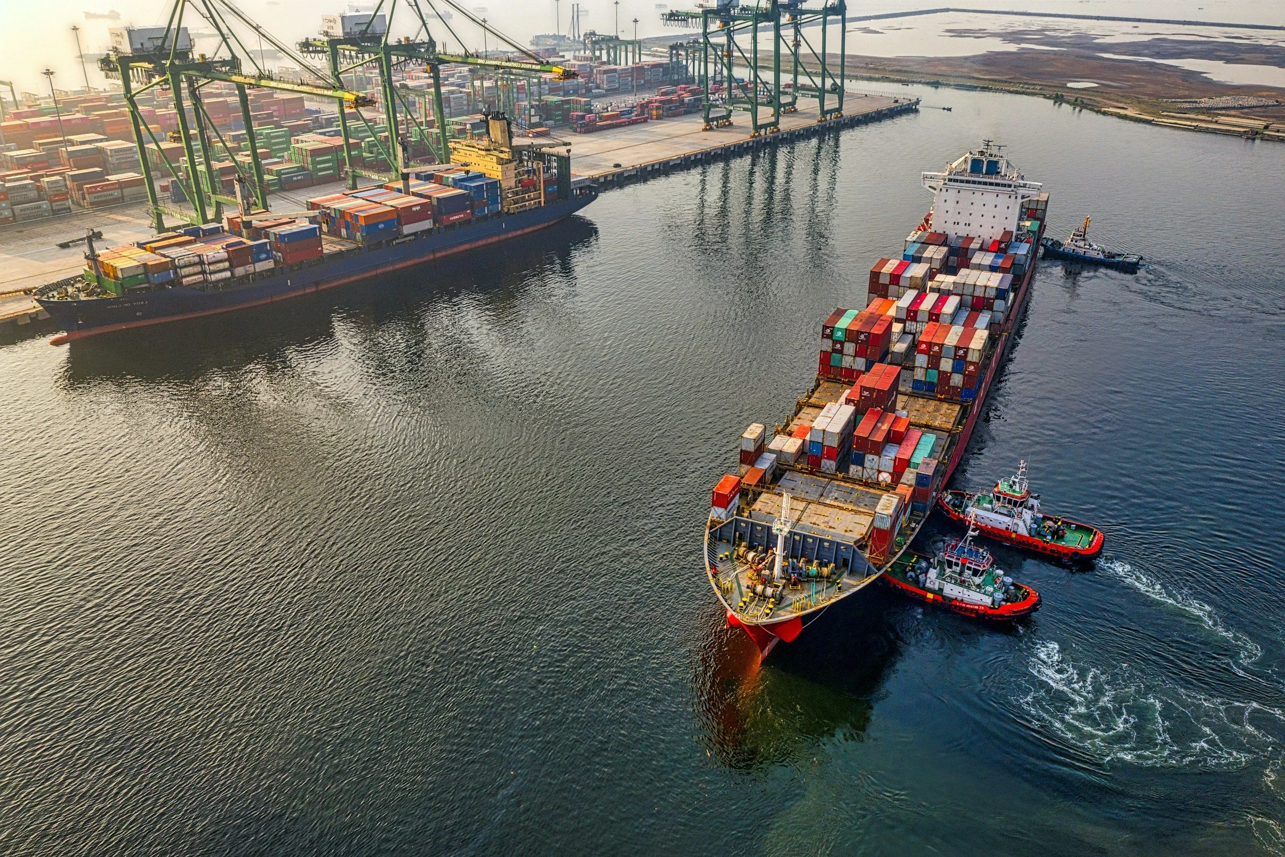
Photo by William07
This is a narrated version of how the Port Congestion Index came to be. If you want a concise summary and key details see Methodology.
Earlier I published an Exploratory post where I used Sentinel-1 SAR imagery to count ships near the Port of Singapore. The original goal was simply curiosity: could satellite radar detect port congestion?
The results were rough, but the signal was there. Major congestion events over the last two years showed up clearly.
The follow-up question was: What if we tracked a basket of major ports around the world on a weekly basis?
To do that I needed a standardized and scalable workflow. There was just one small complication: Apart from a university entry-level programming course 16 years ago, I had never written Python code. Fortunately, these days AI can help.
The end result is a Python script that connects to Google Earth Engine, processes Sentinel-1 imagery and parks the results into Google Drive.
For a while the project progressed suspiciously smoothly. The Orbital Vantage Lab hallmark of repeatedly banging one’s head against the wall only appeared in the end when the results needed refining.
Below is the process of building it.
Development Steps
1. Choose the basket of ports to track
2. Identifying relevant anchorages
3. Automated image collection
4. Automated ship counting
5. Validation
6. Setting a baseline Z-score
7. Future changes
1. Choose the basket of ports to track
“Busiest container ports globally” is not a hard list to find. Six of the top ten are in China. The remaining four are:
Singapore
Busan (South Korea)
Port Klang (Malaysia)
Jebel Ali (UAE)
I wanted a balanced global index and limited China to just two ports:
Shanghai - The world's busiest port
Shenzhen - A key export centre for the Pearl River Delta
I further omitted Malaysia and added:
Nhava Sheva in India
Jebel Ali in the Middle East
Rotterdam and Antwerp in Europe
San Pedro Complex (Los Angeles) and New York in the US
Finally, I included the approaches to Panama Canal and Suez Canal as global shipping choke points.
This brought the index to 12 trackable locations.
2. Identifying relevant anchorages
The first prototype was done quickly. Then it turned into a grind.
Ideally I’d only track anchorages used primarily by container ships, because the Sentinel-1 radar approach cannot distinguish container vessels from tankers or bulk carriers.
To locate these anchorages I analysed AIS density maps from VesselFinder and compared them with published anchorage areas.
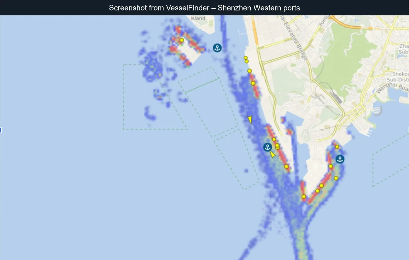
Example AIS density map.
Two problems quickly appeared:
Many ports have multiple anchorages, both near the coast and far offshore
Most anchorages contain mixed vessel types
This means the signal isn’t purely container ships. Singapore and Rotterdam are particularly messy examples. Shenzhen was even worse, as The Pearl River Estuary contains huge amounts of barge traffic and the outer anchorages serve multiple ports simultaneously. But we found a way around this.
The table below shows the key iterative stages. In other words, a lot of polygons were drawn, deleted, redrawn and deleted again while studying how different anchorages in the ports tend to operate.
| Stage | Anchorages | Area |
|---|---|---|
| Prototype | 25 | 660 sq km |
| Peak experimentation | 40 | 1 300 sq km |
| Final version | 28 | 887 sq km |
Transferring and converting data to Google Earth Engine during the iterations was a real pain in the ass. AI told me “This QGIS trick will do what you want in 10 seconds”. After 1 hour of fighting it, I went back to the old method that takes 2 minutes. Progress.
The result is that the PCI is not strictly speaking a container-ship index. However historical checks show that the signal captures major container congestion events quite well. Many ports behave very cleanly.
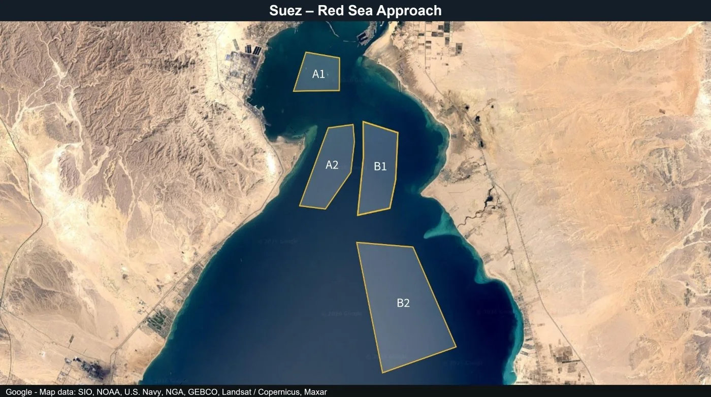
Example anchorage setup in Suez.
3. Automated image collection
This step reused a script developed earlier in The Lab. The logic is:
Look for Sentinel-1 SAR scenes
Identify images that fully cover the anchorages
Select the most recent suitable scene within the last 30 days
The only real change was running this workflow through Python instead of directly inside Earth Engine.
4. Automated ship counting
The ship detection algorithm was also taken from my earlier Singapore experiment. It uses:
Radar intensity thresholds
10-meter resolution data
Morphological closing to merge fragmented radar reflections into single vessels
There is no explicit size-threshold as earlier attempts caused more problems than they solved. Tugboats and small support craft are sometimes detected, but in practice they tend to cluster near larger ships and do not materially distort the counts.
While converting the script to Python, the AI assisting me suggested a much cheaper computational method, and explained its reasoning very confidently. I was intrigued but went for it with healthy trepidation.
I pressed Enter in Python and opened the Google Earth Engine task monitor. Holy moly! Thousands and thousands of EECU seconds (=cost) were flashing before my eyes. I hit “cancel task” and also aborted in Python and prayed for the numbers to stop racking up. They did. I reverted to the old script and went back to tell AI what a wild ride it was.
5. Validation of results
The overall script worked well on the first go and produced a dataset containing:
Anchorage name
Scene timestamp
Detected ship count
The numbers were plausible. But I trusted them about as far as I could throw an emperor penguin. Not that I’ve tried. Some numbers looked too low to be true, like one near-zero count in the Panama Atlantic approach.
Validation was in order. I opened VesselFinder AIS data for the same dates and compared counts. They were broadly consistent, with expected variation from ships arriving and departing. More importantly, I manually inspected the actual SAR images and counted vessels by eye. The satellite images confirmed the numbers and Panama anchorage also was just quiet that day.
The counting algorithm worked. Heavy sea states still need to be tested down the line. Fortunately, container ship radar returns are bright and my detection threshold is quite conservative to not to easily confuse ships with waves.
6. Setting a baseline Z-score
To create a baseline, the script was run across all Sentinel-1 imagery from 2025 for every anchorage. The current congestion value is then calculated as a Z-score deviation from that baseline.
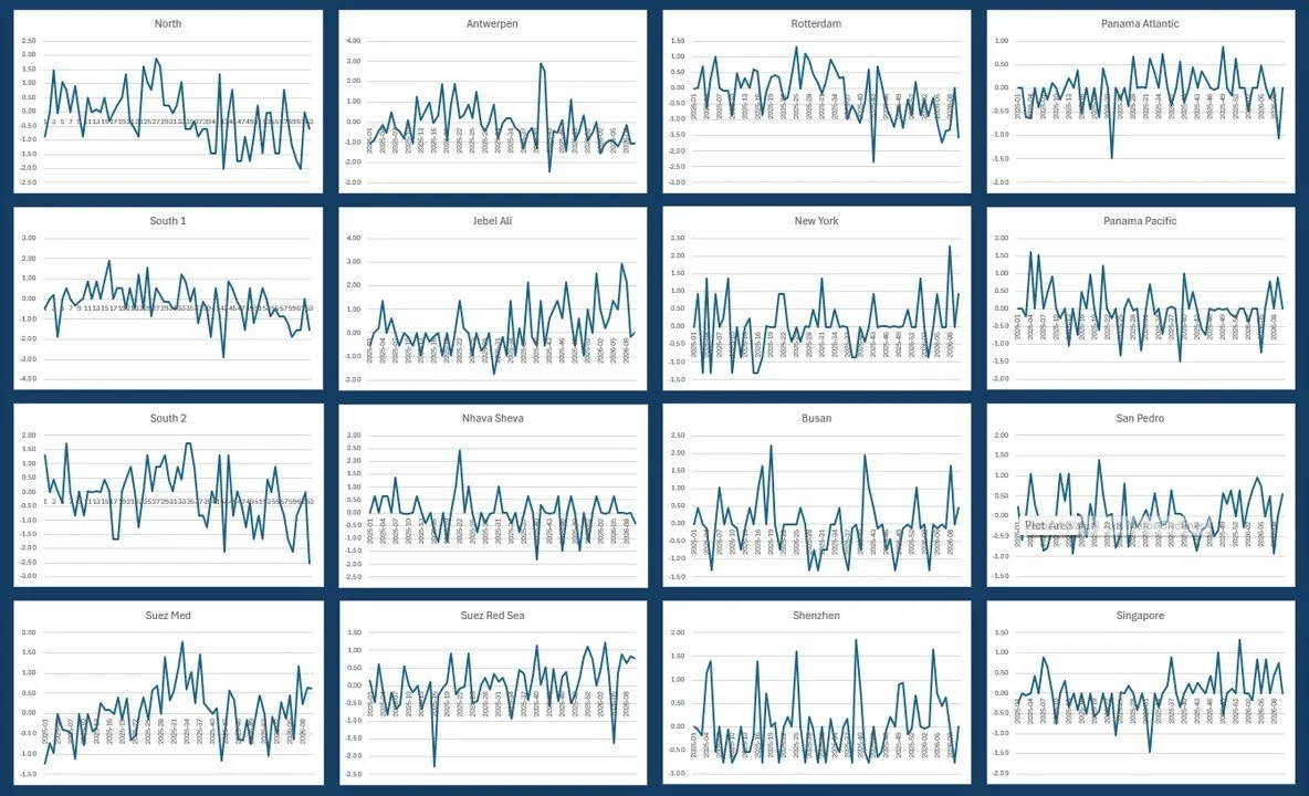
Example results in the development dashboard in excel
The results explain many congestion episodes from last year, though naturally not in a perfect one-to-one relationship. For instance, the impact from winter storm Hernando in February 2026 was immediately evident in the New York data.
This is sufficient for an experimental first release, with validation continuing as new data accumulates.
One complication is that 2025 was already a highly disrupted year, largely due to the Red Sea shipping crisis. If 2026 turns out to be smoother operationally, congestion signals may appear less extreme relative to that baseline.
How the results were ultimately integrated to this site was another hurdle, but mostly a mechanical data process so need to dive deeper into that.
7. Future changes
An index must be stable, so for now the method is locked:
Anchorages remain unchanged
Detection thresholds remain unchanged
As the index is tracked port-by-port, additional ports can be added without affecting existing results in other ports.
Conclusion
This project represents the first transition of an Orbital Vantage Lab experiment into an operational monitoring system.
More importantly for me, it demonstrates something else: I can easily hop to another domain and new technical skills compared to past professional experience, and still get results quickly. Curiosity, persistence and modern tools, not least of which AI, are all it takes.
See you,
Orbital Vantage